Introduction
Differential equations are mathematical equations that describe how a function changes over time. In the case of electricity, they are used to calculate the flow of current through a conductor, resistors, capacitors, and inductors, as well as the analysis of more complex circuits. The flow of electricity in a circuit can be modelled using differential equations that describe the behaviour of voltage and current over time. This study will explore the different differential equations commonly used in electrical circuit analysis, including ordinary and partial differential equations (Kobyzev et al., 2023). The flow of electricity is a very important part of our society. It is responsible for powering devices in our homes and businesses, and it helps us to stay connected to the outside world. The flow of electricity can be complicated, but it can also be modelled using ordinary differential equations (ODEs). This essay will discuss the use of ODEs in calculating the flow of electricity and show how they can be used to solve problems relating to this vital sector of our economy.
Problem statement
The challenges faced in accurately modelling and analyzing electrical circuits require a numerical solution in the calculation of the flow of electricity. Indeed, the use of electrical circuits in modern technology is applied to various electrical appliances. Therefore, using electrical computational equations in the accurate modelling and analysis of the flow of electricity in these circuits is essential for their design, optimization, and efficient operation (Constantin, 2023). However, the behaviour of electrical circuits can be complex and dynamic, and using simple equations makes it challenging to model and analyze using such traditional methods. This has led to the need for more advanced mathematical models and techniques, such as Ordinary Differential Equations (ODEs), to accurately describe and predict the behaviour of these circuits. ODE in mathematical computation is appropriate for the flow of electricity as it employs initial and boundary conditions. Therefore, proper numerical methods for engineering are needed to ensure accurate measurement and estimation of circuit parameters (Kobyzev et al., 2023). Moreover, the emphasis is on the significance of accurate modelling and analysis of electrical circuits, given the potential safety and economic implications of circuit failures or inefficiencies.
Problem solution
Ordinary Differential Equations are commonly used to compute the flow of electricity in various applications, such as electric circuits, power systems, and electromagnetic devices. The solutions that ODE provides are accurate in modelling the circuit and give a meaningful computation of identifying any source of instability. In most cases, the ODE cannot be solved analytically, and numerical methods must be used. This involves discretizing the ODE by dividing the independent variable (usually time) into discrete points. The ODE is then approximated by a set of algebraic equations that relate the values of the dependent variables at each time point. Many numerical methods are available for solving ODEs, such as Euler’s method. The numerical method is implemented to compute the values of the dependent variables at the next time point.
Methodology
This research will use a literature review of case studies in scholarly journals, books and articles to review the use of the ODE in solving the flow of electricity in the circuits. This study will investigate using Euler’s method to provide numerical solutions when employing ODE. The first step is to formulate the ODEs describing the behaviour of the studied electrical system. This involves identifying the relevant variables and parameters, such as voltages, currents, resistances, and capacitances, and formulating the differential equations that relate them (Constantin, 2023). The ODEs can be derived from fundamental physical laws, such as Kirchhoff’s, Ohm’s, and Faraday’s laws. The ODEs are then approximated by a set of algebraic equations that relate the values of the dependent variables at each time point.
Further, the study will use Euler’s numerical methods for solving ODEs. The choice of method depends on the specific characteristics of the ODEs and the application requirements. Once the numerical method has been selected, computer software is in use for the computational analysis of the results. In addition, the computation involves handling boundary conditions, initial conditions, and constraints. Further, after the numerical computation, the results are analyzed to identify if there are any sources of error or instability in the numerical method through visualization by plotting graphs.
Math Modelling
Numerical methods, such as using ODE in solving engineering problems, involve using mathematical models. The flow of electricity computations in the electric circuits can be modelled using ordinary differential equations (ODEs) as the ODE equations compute the behaviour of electricity, such as the electrical variables current, voltage, and resistance over time (Lipovetsky, 2022). Indeed, the ODEs will only be a viable option if they can compute the flow of electricity in a circuit as they are governed by electrical laws such as Kirchhoff’s. The Kirchhoff law state that the sum of the currents entering a node equals the sum of the currents leaving the node, and the sum of the voltages around any closed loop is zero (Al-Ahmad et al., 2020). In addition to the Kirchhoff law, Ohm’s law is the basic equation of electricity that relates voltage, current, and resistance. The Ohms law is represented as V = IR
V is the voltage.
I is the current
R is the resistance.
Ohm’s law equation will be used to model the flow of electricity since it is the most probable equation for a simple circuit with a singular resistor. For example, consider the following circuit: V is the voltage source, R is the resistor, and C is the capacitor. The ODE can describe the behaviour of this circuit:
L(di/dt) + Ri = V(t)
Where L is the circuit’s inductance, di/dt is the current change rate over time, and V(t) is the time-varying voltage supplied by the source. The use of the Euler method in numerically solving the ODE is by approximating the derivative of current concerning time by taking small time steps and computing the change in current over each time step.
For more complex circuits, the ODEs can become more complicated, involving systems of differential equations that describe the behaviour of multiple variables such as current and voltage at different points in the circuit. These systems of ODEs can be solved numerically using matrix methods such as the state-space representation. To develop a mathematical model, let’s consider a circuit that contains a resistor, an inductor, and a capacitor, all connected in series (Bebikhov et al., 2019). The following first-order differential equations can describe the flow of electricity through the circuit:
i’ = -v/R
v’ = -L/C * i – 1/C * q’
q’ = i
i is the current flowing through the circuit.
v is the voltage across the capacitor.
q is the charge stored in the capacitor.
R, L, and C are the circuit’s resistance, inductance, and capacitance, respectively.
To solve these differential equations numerically using Euler’s method;
Take time t=0
Then the current flowing through the circuit is i(0) = 0, the voltage across the capacitor is v(0) = 0, and the charge stored in the capacitor is q(0) = 0. We can then use Euler’s method to compute the values of i, v, and q at subsequent time steps. To apply Euler’s method, time is discretely domain into small time intervals of length h. At each time step n, we compute the values of i, v, and q using the following formulas:
i[n+1] = i[n] + (-v[n]/R) * h
v[n+1] = v[n] + (-L/C * i[n] – 1/C * q[n]) * h
q[n+1] = q[n] + i[n] * h
This process is repeated for each step until the desired endpoint is achieved. The model can be represented in a table as indicated in the example using Euler’s method where the time step of h=0.1
| N | I | V | Q |
| 0 | 0 | 0 | 0 |
| 1 | -0.01 | -0.005 | 0.001 |
| 2 | -0.018 | -0.018 | 0.003 |
| 3 | -0.021 | -0.035 | 0.006 |
| 4 | -0.02 | -0.054 | 0.01 |
| 5 | -0.015 | -0.074 | 0.015 |
| 6 | -0.007 | -0.094 | 0.022 |
| 7 | 0.004 | -0.112 |
Result Analysis
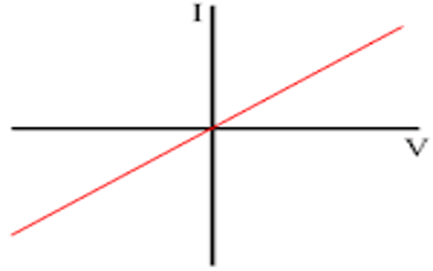
Engineers use the developed mathematical equation model to describe the relationship between current and voltage in different circuit components. However, there is a need to visualize these relationships to better understand how the circuit behaves (Kobyzev et al., 2020). One common graph used in electrical circuits is the voltage-current (V-I) curve, which shows how the voltage across a component changes as the current through the component varies. This curve can be used to determine the component’s resistance, which is the ratio of the voltage to the current. Another useful graph is the power curve, which shows how the power dissipated in a component changes as the current varies (Constantin, 2023). The power dissipated is equal to the product of the voltage and the current, so the power curve can be used to determine the maximum power that the component can deliver.
Here is an example of a V-I graph for a resistor:
Conclusion
The analysis of the results indicates that using ordinary differential equations (ODEs) is adequate in modelling and solving the flow of electricity in various systems. Indeed, the information gathered has illustrated that ODEs provide a mathematical framework for describing how electrical quantities such as voltage, current, and resistance change concerning time or other independent variables. Formulating ODEs to solve the flow of electricity allows researchers to capture the time-varying variable of electrical systems and to simulate how the system will behave in response to multiple time inputs. In addition, ODEs’ flexibility in modelling different types of electrical systems and with the input of numerical computations for a simple circuit or a complex power grid, ODEs are accurate in modelling the flow of electricity.
References
Al-Ahmad, S., Sulaiman, I. M., Mamat, M., & Liza Ghazali, P. (2020). Modified differential transform scheme for solving systems of first-order ordinary differential equations. Journal of Mathematics and Computer Science, 22(01), 73-84. https://doi.org/10.22436/jmcs.022.01.07
Bebikhov, Y. V., Semenov, A. S., Yakushev, I. A., Kugusheva, N. N., Pavlova, S. N., & Glazun, M. A. (2019). The application of mathematical simulation for solving linear algebraic and ordinary differential equations in electrical engineering. IOP Conference Series: Materials Science and Engineering, 643(1), 012067. https://doi.org/10.1088/1757-899x/643/1/012067
Constantin, A. (2023). A uniqueness criterion for ordinary differential equations. Journal of Differential Equations, 342(1), 179–192. https://doi.org/10.1016/j.jde.2022.09.035
Kobyzev, I., Prince, S. J., & Brubaker, M. A. (2020). Normalizing flows: An introduction and review of current methods. IEEE Transactions on pattern analysis and machine intelligence, 43(11), 3964-3979.
Lipovetsky, S. (2022). Mathematical Modeling: Models, Analysis and Applications: by Sandip Banerjee, Boka Raton, FL: Chapman and Hall/CRC Press, Taylor & Francis Group, 2022, 433 pp., $130.00 (hbk), ISBN 978-1-138-49594-4.
 write
write