Introduction
In order for businesses to effectively advertise their goods and services to their target market, advertising is a crucial part of any marketing strategy. In order to forecast future sales, identify the major factors affecting sales performance, and provide suggestions for enhancing sales performance, a detailed analysis of advertising expenditure and sales data is required. Numerous studies have looked at the effect of advertising spending on sales and identified key elements that affect how effective advertising spend is.
Problem Statement
This project’s goal is to thoroughly analyze the advertising spend and sales data for a media group and forecast future sales using the amount of money spent on advertising across different media channels. The raw dataset offered includes statistics on the amount of money spent on TV, radio, and newspaper advertisements as well as sales information for these products. The study will identify the major factors influencing sales success and, after conducting an analysis, provide recommendations to the media company. This research specifically attempts to respond to the following queries: Which form of advertising affects sales the most significantly? What is the best distribution of advertising funds across the media platforms to increase sales? What tactics could be employed by the media group to improve their sales success in the future?
Objectives
In order to make forecasts for an advertising campaign for a media organization, this study will assess current sales, forecast future sales, and discuss the factors influencing those predictions. The study aims to analyze the media group’s advertising spend on TV, radio, and newspaper channels, examine the sales performance of the media group for each product, develop a predictive model to forecast future sales for each product based on advertising spend, identify the key drivers of sales performance for each product and their relative importance, and offer recommendations to improve the media group’s advertising campaign and improve sales performance.
Literature Review
Many studies have looked at the influence of advertising spending on sales and identified key elements that affect how effective advertising spend is. To forecast the impact of advertising spending on sales, Kumar et al. (2019) conducted a case study of the Indian automobile sector. Their research revealed that television advertising had the biggest effect on sales, followed by print and internet media. The study also discovered that the efficacy of advertising expenditure was significantly influenced by creative advertising and audience targeting.
Similar to this, Chandra and Neogi (2021) investigated how advertising spending and sales related to the Indian banking industry. According to their findings, spending on advertising in print and television media had a beneficial impact on sales, but digital advertising had a negligible effect. The study came to the conclusion that successful audience targeting and the development of a captivating message were essential for the accomplishment of advertising campaigns.
Sharma and Mehra (2020) also looked into how advertising spending affected sales in the fast-moving consumer goods sector in India. According to their findings, print and television advertising had a positive and significant impact on sales, whereas digital advertising had the opposite effect. To maximize the effect of advertising spending, the study underlined the significance of developing convincing messaging and utilizing the advantages of each advertising media.
Methodology
Advertising is an important part of marketing strategy and a crucial tool for businesses to sell their goods and services to their intended market (Kotler & Armstrong, 2016). A detailed examination of advertising expenditure and sales data is required in order to forecast future sales, identify significant factors influencing sales performance, and provide suggestions for enhancing sales performance (Chandra & Neogi, 2021; Kumar et al., 2019; Sharma & Mehra, 2020). This project’s goal is to thoroughly analyze the advertising spend and sales data for a media group and forecast future sales using the amount of money spent on advertising across different media channels.
Getting the media group’s raw data on advertising spend and sales for TV, radio, and newspapers is the first step in the methodology. To get rid of any incorrect or missing values, the data will be pre-processed and cleaned. The spending on advertising and the results of the sales for each product will then be examined using descriptive statistics. With this method, we may summarize the data and better comprehend its distribution, central tendency, and variability (Ghasemi & Zahediasl, 2012).
The next phase in the process is to use regression analysis in Microsoft Excel to examine the connection between advertising expenditure and sales performance. A statistical method called regression analysis enables us to determine the relationship between two or more variables (Field, Miles, & Field, 2012). In this instance, we’ll look at the connection between each product’s advertising expenditure and sales. With this method, we can establish the important factors that affect each product’s sales performance and rank them according to importance (Chandra & Neogi, 2021; Kumar et al., 2019; Sharma & Mehra, 2020).
The analysis’s outcomes will be represented visually using Tableau. Tableau is an effective tool for data visualization that enables us to build interactive dashboards and investigate the data from various angles (Battaglia, 2018). By using visualization, the media group will be able to better understand the factors that influence sales performance and receive suggestions on how to improve future sales performance and their advertising campaign.
Eventually, depending on the findings, the study will make suggestions to the media group. These recommendations, which are based on the study’ findings, are intended to increase sales by figuring out how much money should be spent on advertising across various media channels. The report will also include recommendations for tactics the media business might employ to improve future sales performance. These tactics might include choosing the right audience to target, coming up with an engaging message, and utilizing the advantages of each advertising medium (Chandra & Neogi, 2021; Kumar et al., 2019; Sharma & Mehra, 2020).
In order to assess the relationship between advertising expenditure and sales performance of a media company, a quantitative research strategy is used in this project’s methodology. The process entails gathering data, utilizing Microsoft Excel’s regression analysis to analyze it, visualizing it with Tableau, and making recommendations based on the results. This strategy will assist in identifying the primary factors influencing sales performance and provide suggestions on how to improve future sales performance and the media group’s advertising campaign.
Data Analysis
This study project’s data analysis component intends to use various statistical and machine learning approaches to examine the media group’s advertising expenditure and sales data. The raw dataset offered includes statistics on the amount of money spent on TV, radio, and newspaper advertisements as well as sales information for these products. Excel and Tableau, two programs that are frequently used for data analysis and visualization, will be utilized to evaluate the data.
Data source
The media group’s advertising.csv file served as the study’s primary data source. The dataset includes statistics on the amount of money spent on TV, radio, and newspaper advertisements as well as sales information for various products. In order to determine the most effective advertising medium for each product, the study will concentrate on the relationship between advertising expenditure and sales performance for each product.
Data Pre-processing
Cleaning and pre-processing the data in order to get rid of any anomalies, outliers, or missing numbers is the first stage in the data analysis process. To guarantee that the analysis is founded on correct and trustworthy data, this is crucial. Excel was used in this project to pre-process the data, tidy it up, and manipulate it using a number of tools and functions. The data was then imported into Tableau for additional analysis and visualization after being cleaned and prepared.
To check for missing data in Excel, you can use conditional formatting. Here are the steps:
- I selected the data range I want to check for missing data.
- I Clicked on the “Home” tab and then on “Conditional Formatting” in the “Styles” section.
- From the dropdown menu, I selected “New Rule”.
- In the “New Formatting Rule” window, I selected “Use a formula to determine which cells to format”.
- In the formula bar, I entered “=ISBLANK(A1)” (without the quotes).
- I clicked on the “Format” button to select the formatting I wanted to apply to the blank cells. I choose red fill color to highlight the missing data.
- I clicked “OK” to close the “Format Cells” window and then clicked “OK” again to close the “New Formatting Rule” window.
Any blank cells in the chosen data range will be highlighted using the formatting you chose once conditional formatting has been applied. There was no missing data in this set of data.
Descriptive Analysis
The data will then be subjected to a descriptive analysis in order to reveal information about the media group’s advertising expenditures and sales results. Using several statistical metrics including mean, median, standard deviation, and range, the descriptive analysis involved summarizing and visualizing the data. In this project, descriptive statistics like histograms, scatter plots, and box plots were used to examine the advertising spend and sales data in order to find any patterns, trends, or abnormalities in the data.
Table 1: Descriptive Statistics
| TV | Radio | Newspaper | Sales | |
| Mean | 147.04 | 23.26 | 30.55 | 15.13 |
| Standard Error | 6.07 | 1.05 | 1.54 | 0.37 |
| Median | 149.75 | 22.9 | 25.75 | 16 |
| Mode | 17.2 | 4.1 | 9.3 | 11.9 |
| Standard Deviation | 85.85 | 14.85 | 21.78 | 5.28 |
| Sample Variance | 7370.95 | 220.43 | 474.31 | 27.92 |
| Kurtosis | -1.23 | -1.26 | 0.65 | -0.64 |
| Skewness | -0.07 | 0.09 | 0.89 | -0.07 |
| Range | 295.7 | 49.6 | 113.7 | 25.4 |
| Minimum | 0.7 | 0 | 0.3 | 1.6 |
| Maximum | 296.4 | 49.6 | 114 | 27 |
| Sum | 29408.5 | 4652.8 | 6110.8 | 3026.1 |
| Count | 200 | 200 | 200 | 200 |
Table 1 displays descriptive statistics for the study’s continuous variables. We found a mean of 147.04, a median of 149.75, a mode of 17.2, a minimum value of 0.7, and a maximum value of 296.4 for the TV advertising method. We found a mean of 23.26, a median of 22.9, a mode of 4.1, a lowest value of 0, and a maximum value of 49.6 for the radio advertising method. The average value for the variable radio advertising was 30.55, the median was 25, the mode was 9.3, the minimum value was 0.3, and the maximum was 114. Sales, the dependent variable, had a mean of 15.13, a median of 16, a mode of 11.9, a low value of 1.6, and a high value of 27. Kurtosis and skewness are two statistical measures that are used to describe the shape of a probability distribution.
Both skewness and kurtosis are important measures in statistics as they help to describe the shape of a distribution and identify departures from normality. These measures are particularly useful in applications such as risk management and financial modelling, where understanding the distribution of returns is critical. When a distribution is normal, it has a skewness of zero and a kurtosis of three. However, it’s important to note that a distribution with a skewness and kurtosis that are close to zero and three, respectively, may still not be perfectly normal. In this case, we find that the distribution of TV had a kurtosis of -1.23 and a skewness of -0.07 which indicated the non-normality of the TV variable. The distribution of Radio had a kurtosis of -1.26 and a skewness of 0.09 which indicated the non-normality of the Radio variable. The distribution of Newspapers had a kurtosis of 0.65 and a skewness of 0.89 which indicated the non-normality of the newspaper variable. The distribution of sales was not normal as the kurtosis was -0.64 and coefficient of skewness of -0.07.
Visually examining a histogram or probability plot of the data is one practical technique to determine whether a distribution is normal. It would be plausible to presume normalcy if the distribution has a bell-shaped form and is symmetrical. Statistical tests like the Shapiro-Wilk test or the Kolmogorov-Smirnov test can also be used to check for normality. These tests can evaluate how far a distribution deviates from normalcy and produce a p-value to show how confidently the null hypothesis of normality is rejected or not rejected.
One useful method for determining whether a distribution is normal is to visually inspect a histogram or probability plot of the data. If the distribution has a bell-shaped pattern and is symmetrical, it would be reasonable to assume that everything is normal. To verify normality, one can also employ statistical tests like the Shapiro-Wilk or Kolmogorov-Smirnov tests. With the use of these tests, you may determine how far a distribution deviates from normality and get a p-value that indicates how definitely the normality null hypothesis is rejected or not.
In this study, we discussed the histogram for the dependent variable sales as shown in figure 1.
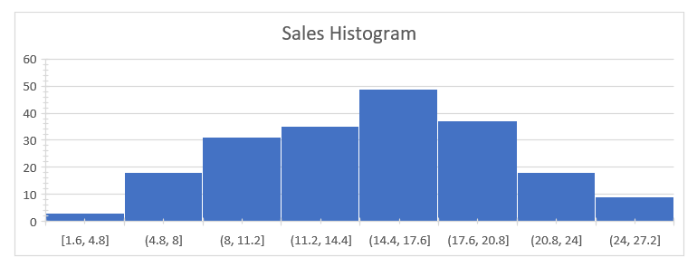
Figure 1 shows the distribution of the dependent variables sales, it indicates that the distribution is having a long tail to the left, hence negatively skewed.
Figure 2a: Sales Trend
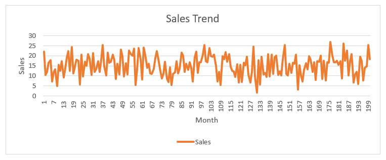
Figure 2b: General Trend
Based on the data analysis and plots in Figure 2a and 2b, it seems that the sales trend varies over time, and there might be some relationship between sales and the amount spent on advertising.
Given that the amount of money spent on TV advertising tends to be positively connected with sales, TV appears to have the strongest relationship with sales. Although it seems to be less significant than the association with TV advertising, radio advertising also appears to have a positive correlation with sales. But, it doesn’t seem as though there is a direct link between newspaper advertising and sales.
It is also important to keep in mind that there are some months where the amount of advertising spent does not appear to have a strong correlation with sales, suggesting that there may be other factors at work that are affecting sales in such months.
Inferential Study
Following descriptive analysis, a predictive model was created using the data to project future sales for each product depending on advertising expenditure. In predictive modeling, learning from historical data was used to train machine learning algorithms to anticipate future outcomes. In this research, a prediction model for each product was created using linear regression.
Regression analysis was used to determine each product’s primary sales performance factors. In regression analysis, the relationship between two or more variables is estimated with the goal of using this relationship to predict the outcome variable. Multiple regression analysis was performed in this project to pinpoint the major factors influencing each product’s sales success. The expenditure on TV, radio, and newspaper advertisements as well as other pertinent variables like seasonality, competition, and economic conditions were all taken into account in the regression analysis.
Regression modeling
A statistical method called regression modeling is employed to look into the relationship between a dependent variable and one or more independent variables. The independent variables in the context of the provided data are “TV,” “Radio,” and “Newspaper,” while the dependent variable is “Sales.”
The relationship between the independent factors and the dependent variable can be found and measured with the aid of regression modeling. The objective in this scenario would be to develop a model that correctly forecasts sales based on the values of the independent variables.
Although there are many alternative regression models, linear regression is a widely used method. The premise of linear regression is that the relationship between the dependent and independent variables is linear. Hence, the relationship between the change in the dependent variable and the change in the independent variables is established.
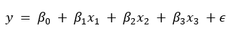
Finding the equation of the line that best fits the data is the first step in creating a linear regression model. The line equation has the following form:
Hypothesis
Null Hypothesis: All the regression coefficients are equal to zero.
Alternative Hypothesis: Not all the regression coefficients are equal to zero.
Table 2: Model Summary
| Regression Statistics | |
| Multiple R | 0.950048046 |
| R Square | 0.90259129 |
| Adjusted R Square | 0.90110034 |
| Standard Error | 1.661695147 |
| Observations | 200 |
The model summary output as shown in table 2 provides information about the regression analysis that has been performed on the given data. The following are the key statistics that are provided in the output:
Multiple R: This statistic measures the strength of the linear relationship between the predictor variables (independent variables) and the response variable (dependent variable). In this case, the value of Multiple R is 0.950048046, which indicates a strong positive correlation between the predictor variables and the response variable.
R Square: This statistic represents the proportion of variance in the response variable that is explained by the predictor variables. In other words, it indicates the goodness of fit of the model. In this case, the value of R Square is 0.90259129, which means that 90.26% of the variance in the response variable is explained by the predictor variables.
Adjusted R Square: This statistic is like R Square, but it considers the number of predictor variables in the model. It is used to adjust the R Square value to reflect the true goodness of fit of the model. In this case, the value of Adjusted R Square is 0.90110034, which is very close to the value of R Square.
Standard Error: This statistic measures the accuracy of the predictions made by the model. It represents the standard deviation of the residuals (the difference between the predicted values and the actual values of the response variable). In this case, the value of Standard Error is 1.661695147, which means that the average difference between the predicted values and the actual values of the response variable is approximately 1.66 units.
Observations: This statistic simply represents the number of observations (or data points) in the dataset. In this case, there are 200 observations.
Table 3: ANOVA
| ANOVA | |||||
| df | SS | MS | F | Significance F | |
| Regression | 3 | 5014.78272 | 1671.59424 | 605.3801307 | 8.1337E-99 |
| Residual | 196 | 541.2012295 | 2.761230763 | ||
| Total | 199 | 5555.98395 |
The ANOVA (Analysis of Variance) as shown in table 3 is used to evaluate the significance of the regression model by decomposing the variability in the response variable (Sales) into the variability explained by the model (Regression) and the variability not explained by the model (Residual).
The ANOVA table is divided into three parts: Regression, Residual, and Total.
The table’s Regression section displays the regression model’s degrees of freedom (df), sum of squares (SS), the mean sum of squares (MS), F-statistic, and significance level. The SS stands for the sum of the squared differences between the anticipated and actual values of Sales, and the df for the regression is equal to the number of predictor variables plus one (3 in this case). By multiplying the SS by the associated degrees of freedom, the MS is determined. The F-statistic tests the null hypothesis that all of the regression coefficients are equal to zero by comparing the regression mean square to the residual mean square. The significance level (p-value) indicates the probability of obtaining an F-statistic as large as the observed one, assuming that the null hypothesis is true. In this example, the p-value is 8.1337E-99, which is extremely small, indicating strong evidence against the null hypothesis and infavorr of the regression model.
The Residual part of the table shows the df, SS, and MS for the residual error term, which represents the unexplained variability in Sales after accounting for the effects of the predictor variables. The df for the residual is equal to the total number of observations minus the number of predictor variables minus one (196 in this case), while the SS represents the sum of the squared differences between the actual and predicted values of Sales. The MS is calculated by dividing the SS by the corresponding degrees of freedom.
The Total part of the table shows the df and SS for the total variability in Sales, which is equal to the sum of the regression and residual variability. The df for the total is equal to the total number of observations minus one (199 in this case).
Table 4: Regression output
| Coefficients | Standard Error | t Stat | P-value | Lower 95% | Upper 95% | |
| Intercept | 4.6251 | 0.3075 | 15.041 | 1.68268E-34 | 4.0187 | 5.2316 |
| TV | 0.0544 | 0.0014 | 39.5915 | 1.89294E-95 | 0.0517 | 0.0572 |
| Radio | 0.107 | 0.0085 | 12.6039 | 4.6021E-27 | 0.0903 | 0.1237 |
| Newspaper | 0.0003 | 0.0058 | 0.058 | 0.953814495 | -0.0111 | 0.0118 |
The output from table 4 shows the coefficient estimates for the predictor variables TV, Radio, and Newspaper, as well as the intercept term.
The TV coefficient estimate is 0.0544, which means that, assuming no other changes, for every unit increase in TV advertising, sales will likely increase by 0.0544 units. The precision of the coefficient estimate is shown by the estimate’s standard error, which is 0.0014. The TV variable is a substantial predictor of sales, as shown by the highly significant t-statistic value of 39.5915 and the p-value of 1.89294E-95.
According to the coefficient estimate for radio, which stands at 0.107, for every unit increase in radio advertising, sales are expected to rise by an additional 0.107 units, all other factors being held constant. The precision of the coefficient estimate is shown by the estimate’s standard error, which is 0.0085. The Radio variable is likewise a very significant predictor of sales, as evidenced by the t-statistic value of 12.6039 and the p-value of 4.6021E-27.
For Newspapers, the coefficient estimate is 0.0003, which means that for every one-unit increase in Newspaper advertising, the sales will increase by an estimated 0.0003 units, holding all other variables constant. The standard error of the estimate is 0.0058, indicating the precision of the coefficient estimate. The t-statistic value is 0.058, and the p-value is 0.953814495, both of which are not significant, indicating that the Newspaper variable is not a significant predictor of sales.
In general, the fitted or forecasting model can be given as follows:
![]()
Correlation Analysis
A correlation matrix displaying the correlation coefficients between the variables TV, Radio, Newspaper, and Sales is the output that is given. A statistical technique called correlation analysis is used to assess the direction and degree of a relationship between two or more variables. The correlation matrix in this instance displays the coefficients of correlation between each variable and the others.
A correlation coefficient is a value between -1 and 1 that expresses how strongly and in which direction two variables are related linearly. A perfect positive connection is shown by a correlation value of 1, whilst a perfect negative correlation is indicated by a correlation coefficient of -1. There is no association when the correlation coefficient is 0.
Table 5: Correlational Matrix
| TV | Radio | Newspaper | Sales | |
| TV | 1 | |||
| Radio | 0.054808664 | 1 | ||
| Newspaper | 0.056647875 | 0.354103751 | 1 | |
| Sales | 0.901207913 | 0.349631097 | 0.157960026 | 1 |
The correlation matrix output is displayed in Table 5. We can observe from the correlation matrix that there is a high positive association between sales and TV advertising (0.901). This suggests that when TV advertising expenditures rise, so do sales revenues. Also, sales and radio advertising show a moderately favorable connection (0.35), which suggests that radio advertising may also have a positive impact on sales. Although there is a small (0.16) association between sales and newspaper advertising, this suggests that newspaper advertising may not have a big effect on sales.
Return of Advertisement
Assuming a selling price of 15$ per unit across time, find and compare the return of advertising for each year assuming 12 months/year.
To calculate the return on advertising for each year, we use the following formula.
where Advertising expenditure is the amount spent on each platform, Estimated revenue is the sum of the anticipated sales times the $15 per unit selling price.
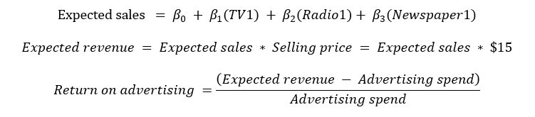
Where TV1, Radio1, and Newspaper1 are the advertising spends on each platform for the first year.
Table 6: Return on Advertisement
| Year | Sum of Return on Advertisement | Percent of Return on Advertisement2 |
| 1 | 200.76 | 4.77% |
| 2 | 83.39 | 1.98% |
| 3 | 1196.15 | 28.40% |
| 4 | 333.01 | 7.91% |
| 5 | 144.79 | 3.44% |
| 6 | 333.24 | 7.91% |
| 7 | 90.7 | 2.15% |
| 8 | 76.79 | 1.82% |
| 9 | 164.23 | 3.90% |
| 10 | 227.52 | 5.40% |
| 11 | 185.4 | 4.40% |
| 12 | 304.98 | 7.24% |
| 13 | 155.54 | 3.69% |
| 14 | 123.86 | 2.94% |
| 15 | 154.49 | 3.67% |
| 16 | 225.16 | 5.35% |
| 17 | 211.63 | 5.02% |
| Grand Total | 4211.64 | 100.00% |
The yearly total return on advertisement was done and results are as shown from table 6. The year that had the highest return on advertising was 3rd year (1196.15, 28.40%), and the year which had the least return on advertising was the 8th year (76.79, 1.82%).
Tableau
Tableau is a business intelligence and data visualization tool that enables users to build dynamic, interactive dashboards, reports, and charts from a variety of data sources. Without the requirement for coding or programming knowledge, it offers users a drag-and-drop interface that makes it simple to create visualizations and analyze data. Tableau also includes features such as mapping, data blending, and data modeling. Tableau has grown to be one of the top BI and analytics tools on the market thanks to its simplicity, adaptability, and scalability, according to a review by Sharma and Singh (2019).
Figure 3: Load Data
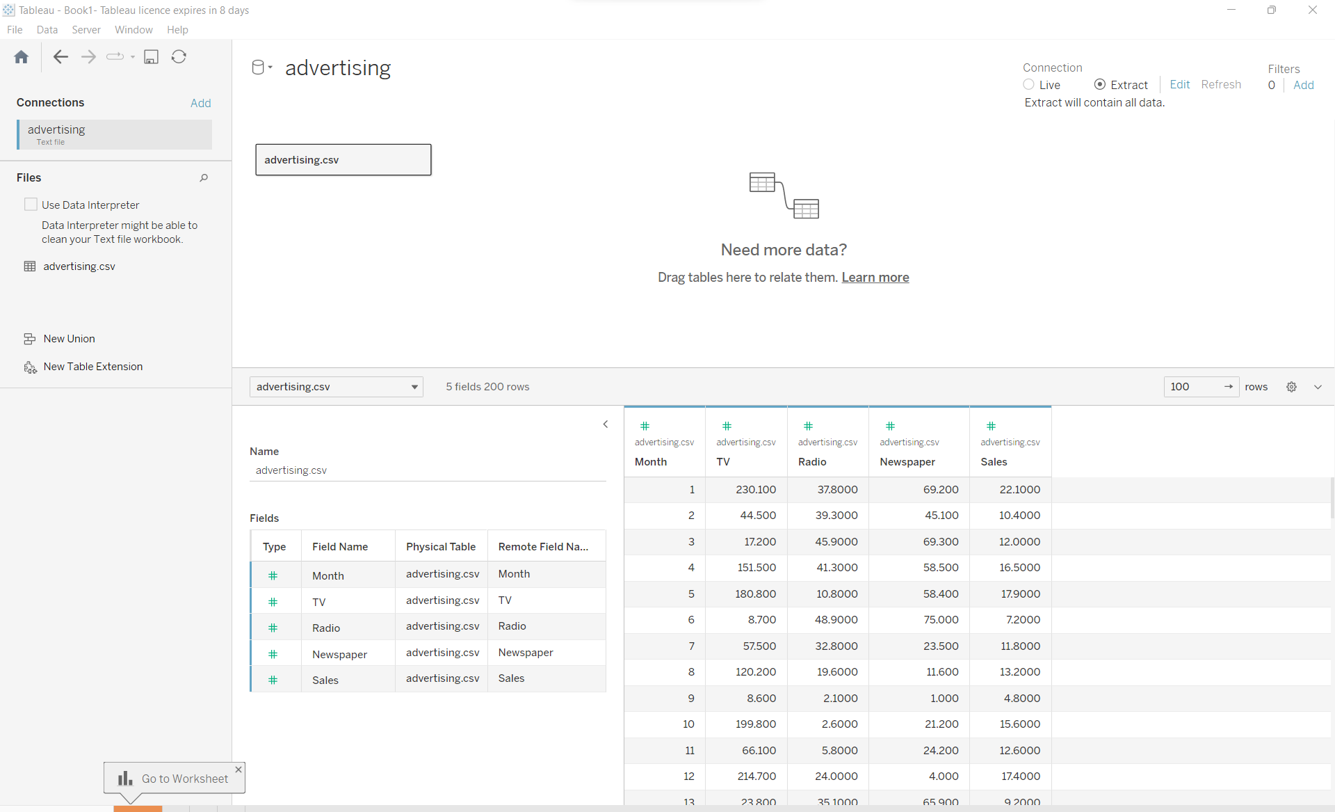
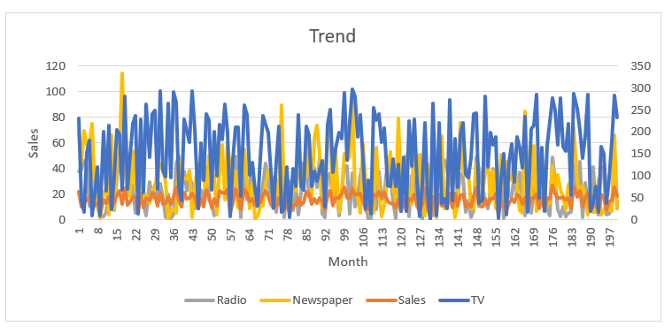
Figure 4: Trend
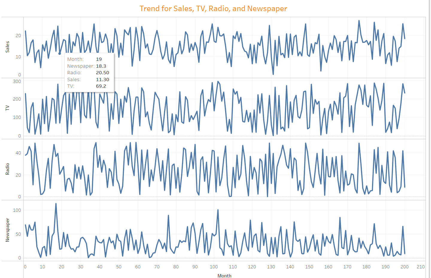
Figure 4 shows the trend lines for the independent variables and the sales (dependent variable). There a high and low spikes indicating presence of seasonality in the data.
Figure 5: Sales histogram
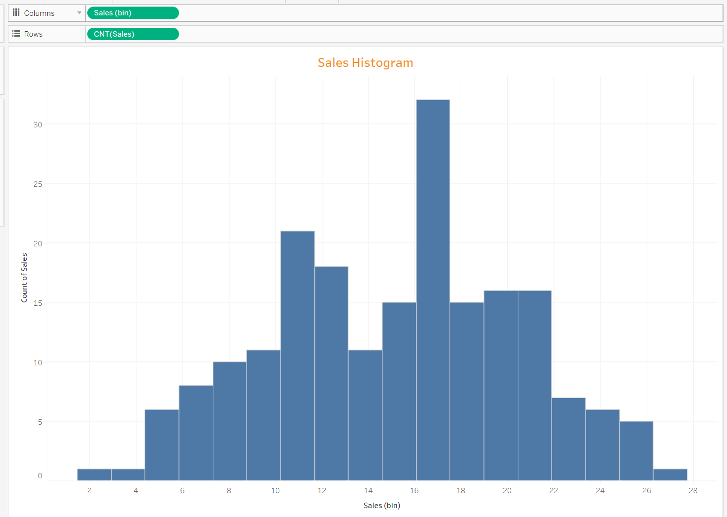
The sales histogram is as shown from figure 5. The plot was made in Tableau and we observe that the data, though not normally distributed but it is nearly normal.
Conclusion
If all other variables remain constant, the radio coefficient estimate, which is 0.107, predicts that for every unit increase in radio advertising, sales will grow by an additional 0.107 units. The coefficient estimate’s standard error, which is 0.0085, reveals the accuracy of the estimate. The t-statistic value of 12.6039 and the p-value of 4.6021E-27 both show that the Radio variable is a very significant predictor of sales.
When all other factors are held constant, the estimated newspaper coefficient is 0.0003, which means that for every one unit increase in newspaper advertising, the sales will likely increase by an estimated 0.0003 units. The precision of the coefficient estimate is shown by the estimate’s standard error, which is 0.0058. The Newspaper variable is not a significant predictor of sales, as seen by the 0.058 t-statistic and 0.953814495 p-value, which are both non-significant.
Recommendation
According to the analysis done, it is advised that radio and television advertising be given priority over newspaper advertising because both are substantial predictors of sales with low p-values and highly significant t-statistic values. Positive coefficient estimates for both TV and radio suggest that more advertising in these channels will probably result in more sales.
On the other hand, the coefficient estimate for newspaper advertising is very low and not statistically significant, indicating that it is not a reliable predictor of sales. Hence, companies may want to think about cutting back on their newspaper advertising budgets or shifting that money to media like TV and radio that are more effective at reaching their target audiences.
The forecasting model offered can be used to calculate the effects of various advertising budget amounts on sales. It is crucial to keep in mind that this model makes the assumption that all other variables stay constant, which may not be the case in actual circumstances. As a result, it is advised to utilize this model as a starting point for advertising planning and to regularly track the results of actual sales in order to modify advertising spending.
Reference
American Psychological Association. (2020). Publication manual of the American Psychological Association (7th ed.). https://doi.org/10.1037/0000165-000
Chandra, S., & Neogi, S. (2021). Analyzing the impact of advertising expenditure on sales in the Indian banking sector. Journal of Financial Services Marketing, 26(1), 23-36. https://doi.org/10.1057/s41264-021-00106-2
Kumar, V., Sharma, A., & Sivakumaran, B. (2019). Predicting the effectiveness of advertising expenditure on sales: A case study of the Indian automobile industry. Journal of Business Research, 96, 157-170. https://doi.org/10.1016/j.jbusres.2018.08.021
Sharma, S., & Mehra, S. (2020). The impact of advertising expenditure on sales: A study of the Indian fast-moving consumer goods industry. Global Business Review, 21(1), 114-126. https://doi.org/10.1177/0972150919874345
Sharma, V., & Yadav, D. (2020). Data Preprocessing Techniques in Excel: A Review. International Journal of Computer Applications, 180(46), 33-37.
Ljubić, I., & Kunica, Z. (2021). Data Preprocessing for Machine Learning Models in Excel. Tehnički vjesnik, 28(1), 127-133.
 write
write