1.0 Abstract
This lab was purposed to find the equilibrium constant in the reaction involving the formation of iron (III) thiocyanate. The lab was based on scientific concepts of Beer’s and the Chartelier’s principles. The constant equilibrium value of 167.10 was reliable as the percentage error was only 25.64 %, indicating high accuracy and reliability in the data sets. The standard error of standard deviation was 1.07 %, indicative that all the equilibrium constants from the different cuvettes were clustered around the average value with no significant outliers, validating the results. The molar absorptivity was 6403.24, measured from a linear plot of absorbance against the concentration of solutions. A square of regression constant, R2, was found to be 0.9942, indicating a very strong and positive relationship between the absorbance measurements and concentrations of the solution. There were minimal errors, and inaccurate feeding of data into the simulator being the only significant error that could have, impacted reliability and accuracy.
2.0 Introduction
The state of chemical equilibrium entails chemical reaction, in which the rate of the forward reaction and backward reaction are equal. At the state of chemical equilibrium, the concentrations of both the reactants and the products tend to remain constant over time. According to the study of Soult (2020), the state of chemical equilibrium will be achieved if the Gibbs free energy of a chemical reaction is zero. A chemical reaction system is at dynamic equilibrium, with both the forward and backward reactions taking place simultaneously. The chemical constant, Kc (Soult, 2020) defines the chemical equilibrium. This constant is expressed as a ration of the concentration of the product and the concentration of the reactants involved in the chemical reaction. The two concentrations are raised to the power of the stoichiometric coefficient.
The chemical equilibrium and chemical reaction with forward and backward reaction is influenced by different factors, including concentration, pressure, equilibrium position, and temperature (Libretext, 2020). The effects of these factors on the chemical equilibrium operate under Le Chatelier’s principle. This principle is instrumental in predicting the changes in all the influencing factors. Le Chatelier’s principle supposes that a chemical reaction under the state of equilibrium, when subjected to any of the influencing factors, adjusts in such a way that it counteracts the effects of the reactant (Libretext, 2020). For instance, increasing the concentrations of reactants in a chemical equilibrium, chemical equilibrium tends to shift towards and in favor of the forward reaction, leading to an increase in concentrations of the products.
A state of equilibrium in a system of the chemical reaction is depicted below:

In the above concentration, if the concentration of reactant A is increased, the reaction will shift towards the right (forward reaction) to maintain the equilibrium status, in line with the principle of Le Chatelier. However, if the concentration of product C is increased, the reaction will shift towards the left (backward reaction) to maintain the chemical equilibrium status. Calculation of the equilibrium constant, Kc involves the determination of equilibrium concentrations of all the products involved in the chemical reaction, then raising them to the coefficients in the balanced equation, then dividing the results with the equilibrium concentrations of all the reactants involved in the chemical reaction raised to the power of coefficients in the balanced equation; as summarized in the following equation, in accordance with Libretext (2020).
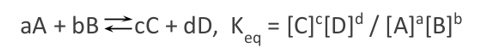
From the above equation;
- A and B are the reactants
- C and D are the products
- Parameters a and b are the coefficients of balancing reactants A and B, respectively.
- Parameters c and d are the coefficients of balancing the products C, and D, respectively.
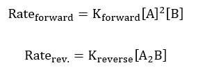
In order to fully describe the chemical equilibrium, the rates of the whole reaction have to be known.
![]()
With respect to this equation of the reaction;
At chemical equilibrium;
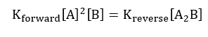
Since the chemical equilibrium for the forward reaction and the reverse reaction are equal, the equivalent chemical equilibrium;
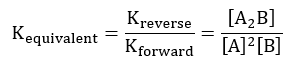
These equations will be used to determine the equilibrium constant for the chemical reaction involving the formation of iron (III) thiocyanate as defined by the following chemical equation.
![]()
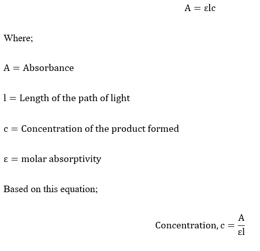
The reaction species in the above equation will chemically combine, reaching chemical equilibrium almost instantly. At the point of equilibrium, there will be the formation of a reddish-brown-orange aqueous solution, with the intensity of the solution being proportional to the concentration. The concentration of this product could be determined through the measurement of the intensity of the solution formed (Libretext, 2020). Additionally, this concentration could be determined through Beer’s law. This law postulates that the absorbance, A varies directly with the length of the path light travels through, molar absorptivity, and the molar concentration of the product formed;
In tdeterminingethe quilibrium constant through this approach, the equilibrium constants of the two reactants, and the product will be required. Additionally, the equilibrium concentration of the product will be needed. This concentration will require prior preparation of the standard solutions of known concentration. The standard solutions would be prepared by mixing small portions of SCN– solution with concentration solution containing Fe3+ in order to shift the chemical equilibrium entirely towards the right side; the side of the product. Through this preparation, it will be possible to determine the equilibrium concentration of the product formed in the experiment.
3.0 Equipment
The main equipment used in conducting this lab activity included:
- Six cuvettes; one for the bank, four for part A of the lab, and one for part B of the lab
- A micropipette and tip
- A SpectroVis Plus
- A 50 mL containing distilled water
- Two 50 mL glass beakers to hold SCN–, and Fe3+
4.0 Method (Steps Followed)
A black USB cable and the spectrophotometer were the first to connect the computer. The logger was then opened and allowed to stand until the spectrum color was observed on the screen.
4.1 Experiment A
An empty cuvette was filled with water to a volume of two-thirds. This cuvette was then placed onto the spectrophotometer holder, with the transparent surface facing the arrow (light). The experiment was then selected by clicking on calibration and ok upon finishing the experiment. The micropipette was then fit with the tip in readiness to fill the first four cuvettes. For cuvette 1, a volume of 1.5 mL Fe3+ was added, followed by 0.6 mL of SCN–, and 0.9 mL of water using the micropipette. For cuvette 2, a volume of 1.5 mL Fe3+ was added, followed by 0.9 mL of SCN–, and 0.6 mL of water using the micropipette. For cuvette 3, a volume of 1.5 mL Fe3+ was added, followed by 1.2 mL of SCN–, and 0.3 mL of water using the micropipette. For cuvette 4, a volume of 1.5 mL Fe3+ was added, followed by 1.5 mL of SCN–, using the micropipette with no addition of water. The micropipette was rinsed with water, and disposed into the waste bin between solutions. The blank (distilled water) was removed from the spectrophotometer, and cuvette #1 was added before pressing collect. After that, cuvette #2 was removed, and cuvette #3 was added before pressing on collect. After that, cuvette #3 was removed, and cuvette #4 was added before pressing on collect. The data obtained was exported as the SCV.
4.2 Experiment B
The data icon was then pressed to clear all the data. Another cuvette was then selected and filled with 0.3 mL SCN– using the micropipette. The tip of the cuvette was then rinsed with distilled water, then disposed into a waste bin. A volume of 2.7 mL concentrated Fe3+ was added into the same cuvette using the same micropipette but had to be rinsed with distilled water. The cuvette was then placed onto the spectrophotometer, and the collet option was pressed. The concentrated Fe3+ solution was removed from the cuvette, and an equal amount of nitric acid was added to the same cuvette (750 microliters). The cuvette was then closed using a cuvette lit, then gently flipping the cuvette upside down to ensure uniform mixing. The cuvette was then returned to the spectrophotometer, and the collected option was processed to store the latest run. A volume of 1000 microliter was then removed from the cuvette and replaced with 1000 micro liter of the nitric acid solution. The cuvette was then closed using a cuvette lit, then gently flipping the cuvette upside down to ensure uniform mixing. A volume of 750 microliters of copper sulfate solution was removed twice from the cuvette, and an equal volume of nitric acid was added into the same cuvette. The cuvette was then closed using a cuvette lit, then gently flipping the cuvette upside down to ensure uniform mixing. The cuvette was then returned to the spectrophotometer, and the collected option was processed to store the latest run. The data obtained was exported as the SCV.
5.0 Results
The volumes of the reactants prepared in the experiment were presented in tables 1, and 2 below. The last column shows the measured absorbance values at each of the cuvettes.
Table 1: FeSCN Calibration Data Sets (Part A)
| Vol/ FeIII-SCN | Vol+(0.1M HNO3) | Concentration/M | Absorbance@439.9nm |
| 0 | 0 | 2.00E-04 | 1.2320 |
| 0.75 | 0.75 | 1.50E-04 | 0.8819 |
| 1 | 1 | 1.00E-04 | 0.5120 |
| 1.5 | 1.5 | 5.00E-05 | 0.2404 |
| 1.5 | 1.5 | 2.50E-05 | 0.1210 |
Table 2: Volumes of the Prepared Solutions (Part B)
| Cuvette | Vol/[Fe3+]/ml | Vol[SCN–]/ml | Vol/H2O | Absorbance @451.2nm |
| #1 | 1.5 | 0.6 | 0.9 | 0.346 |
| #2 | 1.5 | 0.9 | 0.6 | 0.511 |
| #3 | 1.5 | 1.2 | 0.3 | 0.669 |
| #4 | 1.5 | 1.5 | 0 | 0.822 |
The concentrations of the two reactants in the experiment were such that;
[SCN–]: 2.00E-3
[Fe3+]: 2.00E-3
The values of concentrations and absorbance measurements were used to create a linear graph of absorbance against the concentration of solutions in the Microsoft Excel application, as depicted in the figure below.
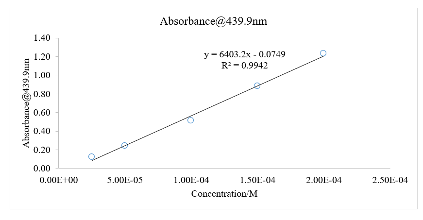
Figure 1: A linear Graph of Absorbance against Concentration at a Wavelength of 439.9 nm
The relationship between absorbance and the concentration of a solution is defined by the following equation, in line with Beer’s law;
![]()
Thus, with respect to the graph of A against c in figure 1, the slope of the graph corresponds to the product of molar absorptivity and the length of the path of light.
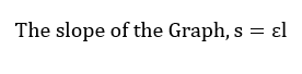
The length of light will be assumed to be 1 cm. Thus, the molar absorptivity was found to be equivalent to the slope of the graph;
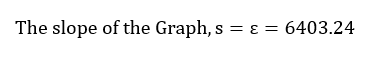
This value will be utilized in the succeeding steps to calculate the standard concentration of the product formed in the experiment.
The standard absorbance of the product formed was read from the spectrophotometer as the maximum absorbance in the first run, such that;
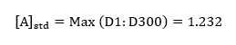
Using the volumes presented in table 1, and the concentrations of each of the two reactants, the concentrations of the equivalent reactants could be calculated;
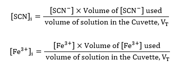
For sample calculations, considering the volumes of reactants in the cuvette, #1;
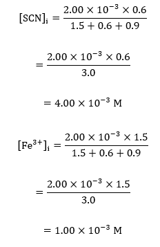
These calculations were extended to the rest of the data values, and all the results obtained were recorded into the following table of values;
Table 3: Equivalent Concentrations of the Reactants
| Cuvette | [SCN– ]i | [Fe3+]i |
| #1 | 4.00E-04 | 0.001 |
| #2 | 6.00E-04 | 0.001 |
| #3 | 8.00E-04 | 0.001 |
| #4 | 1.00E-03 | 0.001 |
The concentration of the product formed in the experiment will be based on Beer’s law;
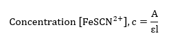
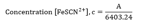
The length of light will be assumed to be 1 cm, and the molar absorptivity has been determined from the linear graph in figure 1 as 6403.24. Thus;
For sample calculations, the considering the absorbance measured in the cuvette, #1;
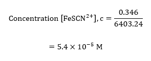
These calculations were extended to the rest of the absorbance values in the different cuvettes, and all the results obtained were recorded into the following table of values;
Table 4: Concentrations of the Equivalent Product
| Cuvette | [FeSCN]2+ |
| #1 | 5.40E-05 |
| #2 | 7.98E-05 |
| #3 | 1.05E-04 |
| #4 | 1.28E-04 |
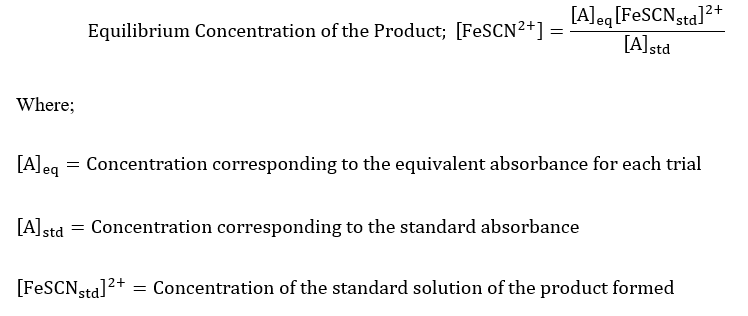
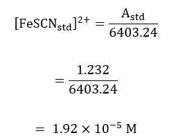
The standard concentration of the product was calculated in the same approach but using the standard absorbance;
The next calculations were for the free thiocyanate concentrations and iron (III) ions. They were calculated as the difference between the molar concentrations of the equivalent thiocyanate, and iron (III) ions and the concentration of the iron (III) thiocyanate ions;
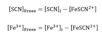
For sample calculations, the considering the measurements of concentrations in cuvette, #1;
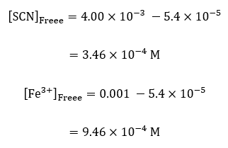
Table 5: Free Ions Concentrations
| Cuvette | [SCN– ]free | [Fe3+]free |
| # 1 | 3.46E-04 | 9.46E-04 |
| # 2 | 5.20E-04 | 9.20E-04 |
| # 3 | 6.95E-04 | 8.95E-04 |
| # 4 | 8.72E-04 | 8.72E-04 |
The values obtained in table 4, and the general equation was used to calculate the equilibrium constant of the reaction;
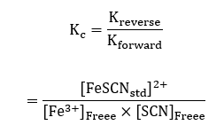
For sample calculations, the considering the measurements of concentrations in cuvette #1;
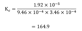
This formula was used with the rest of the concentration pairs in the different cuvettes, and all the results were obtained from the calculations used to record table 5 below.
Table 6: Equilibrium Constant at different Concentrations of the Iron (II) and Thiocyanate Ions
| Cuvette | [SCN– ]free | [Fe3+]free | Equilibrium Constant, Kc |
| # 1 | 3.46E-04 | 9.46E-04 | 164.9 |
| # 2 | 5.20E-04 | 9.20E-04 | 166.7 |
| # 3 | 6.95E-04 | 8.95E-04 | 167.8 |
| # 4 | 8.72E-04 | 8.72E-04 | 169.1 |
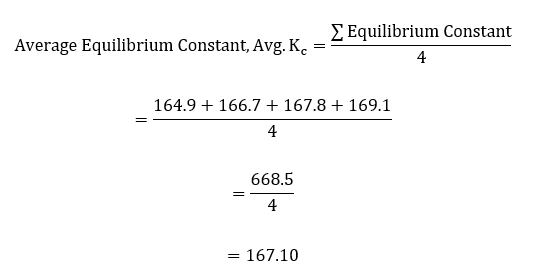
The average equilibrium constant was then calculated using the values in the last column of table 5 above;
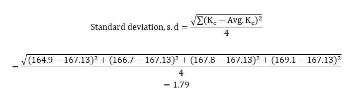
The average value obtained was then used to work out the standard deviation of equilibrium constants;
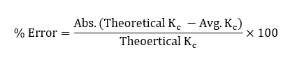
The percentage error in the equilibrium constant was calculated using the theoretical equilibrium constant and the average experimental value of the equilibrium constant;
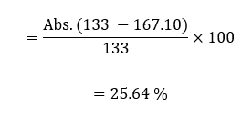
The theoretical equilibrium constant of iron (III) thiocyanate is 133 (de Berg, 2019). Using this value, it was possible to calculate the percentage error:
The standard error was then calculated as a function of the standard deviation and the average value of the experimental equilibrium constant;
6.0 Discussion
This lab activity aimed to find the equilibrium constant of the reaction involving the formation of iron (III) thiocyanate. In the first part of the lab, the FeSCN solution was calibrated. The calibration curve was found to be very reliable since the initial concentrations of the reactants had been accurately measured using the online simulator of the lab. The values of absorbance of each of the solutions in the cuvettes were measured using the same simulator spectrophotometer software. This factor decreases the possibility of random human perception errors. Absorbance measurements were taken at a predefined wavelength, then graphed against the concentrations of solutions in the different cuvettes. Upon graphing, it was possible to determine the molar absorptivity of the reaction as the slope of the linear graph, with the imploration of Beer’s law. The value was found to be 6403.24. The square of the regression constant, R2, was 0.9942, on a scale of between 0 and 1, indicating a very strong and positive relationship between the absorbance measurements, and concentrations of the solution. Additionally, this value showed a high measure of accuracy and reliability in the experimental results. Most of the data points were found to be along the trend line, a further mark or reliability, both in the results and the method used to conduct the lab activity.
In the second part of the lab activity (part B), the equivalent chemical equilibrium of the reaction was calculated. The equivalent equilibrium constant had been expected to be reliable, considering that the entire experimental activity was conducted through an online simulation, limiting the possibility of random and systematic errors. In determining this equilibrium constant, the samples in the different cuvettes were not forced to shift the equilibrium towards the left or the right side of the equation to ensure standard conditions. The constant equilibrium value of 167.10 was reliable as the percentage error was only 25.64 %. Additionally, the standard error of standard deviation was 1.07 %, indicative that all the equilibrium constants from the different cuvettes were clustered around the average value with no significant outliers, validating the results.
This lab had minimal chances of experimental errors since it was conducted entirely through an online simulation. This approach reduced the possibility of systematic errors associated with calibrating and taking measurements using different equipment and the random errors attributed to human perceptions in an in-person experimental approach. However, there may have slight random errors in the simulation. Inaccurate entering of different values, including the volume of solution in the simulation, could have impacted the reliability and accuracy of the measured results and the calculated value of the equilibrium constant.
7.0 Conclusion
This lab activity aimed to find the equilibrium constant in the reaction involving the formation of iron (III) thiocyanate. This constant was determined based on Beer’s law and Chartelier’s principle. Beer’s law enabled effective and accurate determination of the molar absorptivity of the solution (6403.24). The accuracy of this value was shown by a high value of R2 and linearity of the scatterplot of absorbance against the concentration of iron thiocyanate solution. Chartelier’s principle was used to calculate the equilibrium constant, a value found to be 167.10 with a percentage error was only 25.64 % from the theoretical value and a standard error of 1.07 %, indicating high accuracy and reliability. There were minimal errors, with an inaccurate entry of different values into the simulator being the major possible error that could have, impacted reliability and accuracy. This error can be avoided by ensuring accuracy in calibration and feeding different values into the online simulator.
8.0 References
de Berg, K. C. (2019). The Iron (III) Thiocyanate Reaction. In SpringerBriefs in Molecular Science. Springer International Publishing. https://doi.org/10.1007/978-3-030-27316-3
Libretext. (2020, January 13). 2: Determination of an Equilibrium Constant. Chemistry LibreTexts. https://chem.libretexts.org/Courses/Saint_Marys_College_Notre_Dame_IN/Chem_122L%3A_Principles_of_Chemistry_II_Laboratory_(Under_Construction__)/02%3A_Determination_of_an_Equilibrium_Constant
Soult, A. (2020, August 5). 8.2: Chemical Equilibrium. Chemistry LibreTexts. https://chem.libretexts.org/Courses/University_of_Kentucky/UK%3A_CHE_103_-_Chemistry_for_Allied_Health_(Soult)/Chapters/Chapter_8%3A_Properties_of_Solutions/8.2%3A_Chemical_Equilibrium
 write
write