Introduction
Data pretreatment and feature engineering are essential before data analysis or predictive modelling. They involve transforming unprocessed data into a format that can be effectively and efficiently processed. The level of effort devoted to these procedures directly affects the data’s quality and utility. This endeavor will utilize a dataset comprising daily weather observations from diverse regions across Australia spanning approximately ten years. Due to its wealth and diversity, the dataset is an ideal subject for showcasing an array of feature engineering and data preparation methodologies.
The objective of this endeavor is to conduct extensive data cleansing and preprocessing prior to conducting feature engineering. This process will not only optimize the data for subsequent predictive tasks and analytics, but it will also enhance the predictive efficacy of the features. Each phase of the data preprocessing and feature engineering procedure will be examined in detail in the following sections, with thorough justifications and explanations for every decision and action.
Dataset description
The dataset for this assignment comprises daily weather observations from multiple Australian weather stations spanning approximately ten years. A decade’s worth of data collected from these stations offers a comprehensive depiction of the weather patterns in Australia. The dataset contains variables such as temperature, humidity, wind speed, and precipitation, representing diverse facets of the weather. By associating each observation with a distinct date and location, it becomes possible to track the evolution of weather patterns throughout Australia and time.
In the following section we handle the data preprocessing and cleaning process. This will entail dealing with missing values, outliers, and duplicate records and putting the data into an analysis-ready format.
Phase 1: Data preprocessing and cleaning
Any data analysis or predictive modelling work requires data pretreatment and cleaning. It entails converting raw data into a format that can be worked with efficiently and effectively. The amount of effort invested into these procedures directly affects the data’s quality and usefulness. In this project, we will be working with a dataset in this project that includes around ten years of daily weather observations from various areas across Australia (Joshi & Patel, 2021). The dataset is rich and diverse, making it ideal for demonstrating a variety of data pretreatment and cleaning approaches.
This project aims to perform a thorough data cleaning and preprocessing procedure. Not only will this prepare the data for downstream analytics and predictive jobs, but it will also improve the predictive value of the features. We will walk through each step of the data preprocessing and cleaning process in the sections that follow, providing extensive explanations and arguments for each decision and action performed.
Handling missing values
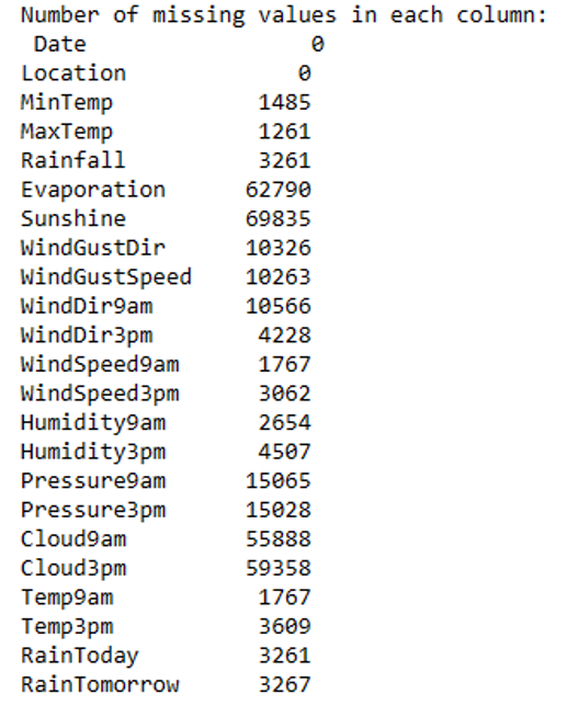
Before starting with preliminary data, we first identify non-important areas. The number of missing values in each row is large enough to be solved. The figure below shows the rows with missing values and calculated missing values.
To eliminate missing values, we divided the dataset into numerical and categorical columns. This is because the way missing values are handled varies by data type. We used median imputation for the numerical columns. This method substitutes missing values with the column’s median value. When dealing with numerical data, the median is typically better than the mean because it is less sensitive to outliers.
We employed mode imputation for the categorical columns. This method substitutes missing values with the column’s mode (most frequent value). This is a standard method for dealing with missing categorical data. After using these imputation approaches, we ended up with a clean dataset with no missing values. Following handling, the number of missing values in each column is as follows:
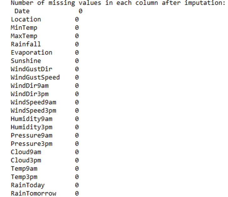
This was an essential step in ensuring our dataset was complete and ready for future research. The following section will review how we dealt with outliers in the dataset.
3.2 Handling outliers
Outliers can drastically affect the outcomes of the data analysis and statistical modelling. Therefore, it is vital to detect and treat outliers effectively.
Initially, we discovered 12 columns with probable outliers. For simplicity, we only analyzed numerical columns as they are more likely to include outliers that can be found using statistical approaches. We utilized the Z-score approach to identify outliers. The Z-score measures how far away a data point is from the mean. It is measured in terms of standard deviations from the mean. As a rule of thumb, a Z-score of more than three or less than -3 is considered an outlier. After identifying the outliers, we addressed them by eliminating the rows with a Z-score of more than 3. This is a frequent approach to controlling outliers, especially when the dataset is large enough that eliminating any data will not cause a major loss of information.
After adopting this outlier treatment strategy, the number of columns containing outliers dropped to 3. This suggests that our strategy effectively minimized the dataset’s outliers. In the next section, we will examine how we dealt with duplicate records in the dataset.
3.3 Dealing with duplicate values
We searched for duplicate entries inside our dataset. If a record possessed identical values for all features as another record, it was considered a duplicate. Upon examining our dataset, we determined no instances of duplicate records. This indicator is reliable as each entry in our dataset is unique and represents an individual observation.
The lack of duplicates in our dataset streamlines the preprocessing procedure while guaranteeing the integrity of our dataset and the validity of our following study. In the subsequent part, we will elucidate the process of transforming the data into a suitable format for analysis.
3.4 Data transformations
Data transformation is an essential stage in the preprocessing of data. It entails turning the data into a format that can be worked with efficiently and effectively. We had to deal with two types of data transformations in our case:
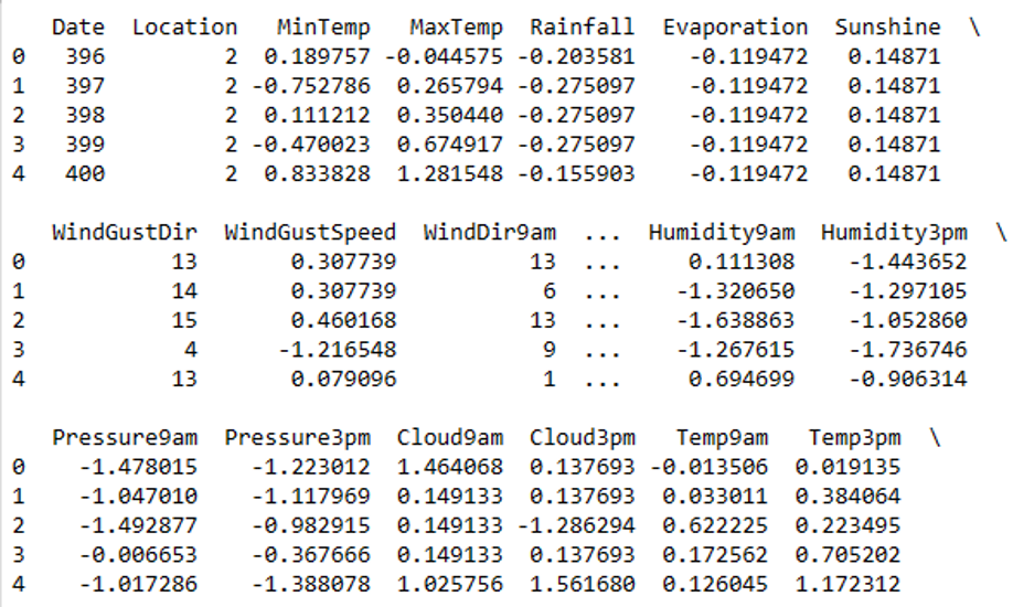
Creating Numerical Representations from Categorical Variables: Categorical variables can only have one of a few possible values. Our dataset had multiple categorical variables, including WindGustDir, WindDir9am, WindDir3pm, RainToday, and RainTomorrow. We translated these variables into numerical representations to make them more amenable to analysis and modelling. For this, we employed label encoding. Label encoding assigns a number to each distinct category in a feature. This method is straightforward and effective for changing categorical values.
Numerical characteristics scaling: Numerical characteristics frequently have an extensive range of values. Because some algorithms are sensitive to the magnitude of the input features, this can present issues when undertaking data analysis or predictive modelling. We scaled the numerical characteristics in our dataset to remedy this. For this, we used conventional scaling. The features are transformed using standard scaling with a mean of 0 and a standard deviation of 1. This ensures that all characteristics have the same scale without distorting or losing information due to variances in the range of values.
We verified that our data was acceptable for downstream analytical and prediction tasks by changing it in this manner. This phase was critical in assuring the efficacy and precision of our following analysis (Hendrycks et al., 2019). The following figure displays the first few rows of the transformed dataset.
In the following section, we will go over the feature engineering process, in which we will construct new features and implement dimensionality reduction, binning, discretization, and feature scaling.
Feature engineering
Feature engineering is an essential stage in data analysis and predictive modelling. It entails generating new features from existing ones, altering old ones to make them more suited for modelling, and selecting the most relevant features for the job.
Feature engineering aims to increase machine learning model performance by supplying high-quality, informative features. Creating interaction features, extracting information from text, and binning numerical variables are all examples of strategies that can be used. We will conduct numerous feature engineering activities in this assignment, such as developing new features, implementing dimensionality reduction, binning and discretization, and feature scaling (Rawat & Khemchandani, 2017). Each job will help improve our features’ predictive power and the performance of our downstream analytics and predictive tasks.
Creating new features
It is standard practice in machine learning and data analysis to create new characteristics from current ones. It can help to improve the model’s predictive power and identify hidden patterns in the data.
We added the following additional features to our dataset:
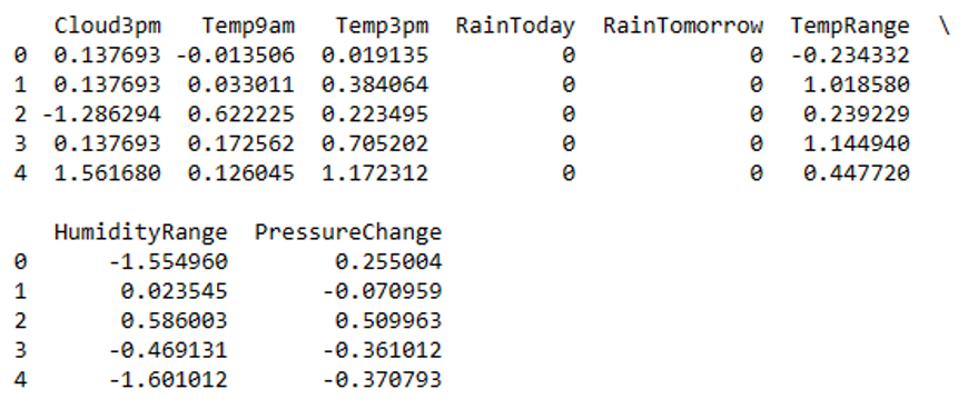
Temperature Range: This feature captures the temperature range throughout the day, which may be beneficial for predicting weather trends. It is calculated as the difference between the maximum and minimum temperatures.
Humidity Range: Like the temperature range, this component captures the humidity range throughout the day. The difference between Humidity9am and Humidity3pm is used to calculate it.
Pressure shift: This feature records the shift in air pressure from morning to afternoon, which may indicate certain weather trends. It is determined as the difference between 9 a.m. and 3 p.m. pressures.
These new features add information to the original dataset that was not explicitly available, potentially increasing the effectiveness of our downstream analytical and predictive activities. The following figure displays the first few columns of the newly created features of the dataset.
The implementation of dimensionality reduction strategies will be discussed in the next section.
4.2 Dimensionality reduction
Dimensionality reduction is a strategy for reducing the number of variables in a dataset. It is especially beneficial when dealing with datasets with many features because it can assist in making the data more comprehensible, enhance model performance, and prevent overfitting.
However, in our instance, the dataset has limited features. As a result, we may not need to conduct this step. When determining the preprocessing and feature engineering processes, examining the individual dataset’s features is crucial (Rawat & Khemchandani, 2017). The implementation of binning and discretization techniques will be covered in the next section.
4.3 Binning and discretization
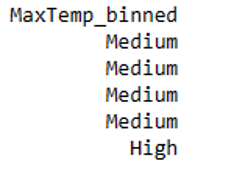
Binning and discretization is a method of converting continuous numerical variables to categorical counterparts. This can be useful when the exact numerical value is less relevant than the range within which it falls. We opted to discretize the MaxTemp column in our dataset into three bins: low, medium, and high (Navas-Palencia, 2020). This modification can simplify the data and make it easier to comprehend while keeping the overall temperature trend.
MinTemp, Rainfall, Evaporation, WindGustSpeed, WindSpeed9am, WindSpeed3pm, Humidity9am, Humidity3pm, Pressure9am, and Pressure3pm are all suitable variables for binning and discretization in addition to MaxTemp. All of these are continuous variables that might be translated into categorical counterparts. The following snippet shows the first few rows of the new max temp column after binning.
4.4 Feature scaling
Feature scaling is a technique for standardizing independent variables or data features. It is often carried out during the data preparation step. Many machine learning techniques require feature scaling as a preprocessing step. It can help to normalize data inside a specific range and can also aid in speeding up algorithm calculations. We used feature scaling in our dataset to ensure all features had the same scale (Rawat & Khemchandani, 2017). This is especially essential for machine learning algorithms sensitive to input feature scale.
We exhibited Min-Max Scaling as well as Standardization: Min-Max Scaling: Rescales the features to a defined range, often 0 to 1. The new value of a feature is computed by subtracting the feature’s value from the minimum value and dividing the result by the range of the feature’s values.
Standardization: This approach standardizes features by reducing the mean and scaling to unit variance. The new value of a feature is computed by subtracting the feature’s value from the mean value and dividing the result by the standard deviation of the feature’s values.
By employing feature scaling, we guaranteed that no feature dominated others in our downstream analytics and prediction jobs, potentially improving their performance. We have now completed the feature engineering process. The following part will summarize our findings and discuss how important these procedures are for downstream analytics and predictive jobs.
Conclusion
This study uses data preprocessing and feature engineering on a dataset, including around ten years of daily weather observations from several places across Australia. We began with data pretreatment and cleaning, including missing values, outliers, and duplicate records. The data was then translated into an analysis-ready format by transforming categorical variables into numerical representations and scaling numerical features.
Following that, we went on to feature engineering, where we developed additional features that applied dimensionality reduction, binning, discretization, and feature scaling, among other things. These processes improved our features’ predictive power and the performance of our downstream analytics and predictive jobs. We have proved the relevance of data pretreatment and feature engineering in preparing data for analysis and modelling through this approach. These processes are critical for assuring the efficacy and accuracy of our subsequent analysis and prediction jobs. They aid in discovering hidden patterns in data, enhancing machine learning models’ performance, and producing more accurate and dependable outputs.
This task has given us hands-on experience in data preparation for analysis and modelling. It has emphasized the difficulties of working with real-world data and the significance of rigorous data pretreatment and feature engineering. We hope the methodologies and strategies mentioned in this study will be valuable in future data analysis and predictive modelling assignments.
References
Hendrycks, D., Mu, N., Cubuk, E. D., Zoph, B., Gilmer, J., & Lakshminarayanan, B. (2019). Augmix: A simple data processing method to improve robustness and uncertainty. arXiv preprint arXiv:1912.02781. https://www.bing.com/ck/a?!&&p=769d987dec869693JmltdHM9MTcwMTEyOTYwMCZpZ3VpZD0xYWE5YTM2YS0zZTAwLTY5NWEtMzMxMS1iMGEzM2Y4NzY4NGQmaW5zaWQ9NTE5Mg&ptn=3&ver=2&hsh=3&fclid=1aa9a36a-3e00-695a-3311-b0a33f87684d&psq=Hendrycks%2c+D.%2c+Mu%2c+N.%2c+Cubuk%2c+E.+D.%2c+Zoph%2c+B.%2c+Gilmer%2c+J.%2c+%26+Lakshminarayanan%2c+B.+(2019).+Augmix%3a+A+simple+data+processing+method+to+improve+robustness+and+uncertainty.+arXiv+preprint+arXiv%3a1912.02781.&u=a1aHR0cHM6Ly9hcnhpdi5vcmcvYWJzLzE5MTIuMDI3ODE&ntb=1
Joshi, A. P., & Patel, B. V. (2021). Data preprocessing: the techniques for preparing clean and quality data for data analytics process. Oriental journal of computer science and technology, 13(0203), 78-81. https://www.bing.com/ck/a?!&&p=26a03ead22bd7e58JmltdHM9MTcwMTEyOTYwMCZpZ3VpZD0xYWE5YTM2YS0zZTAwLTY5NWEtMzMxMS1iMGEzM2Y4NzY4NGQmaW5zaWQ9NTE5OA&ptn=3&ver=2&hsh=3&fclid=1aa9a36a-3e00-695a-3311-b0a33f87684d&psq=Joshi%2c+A.+P.%2c+%26+Patel%2c+B.+V.+(2021).+Data+preprocessing%3a+the+techniques+for+preparing+clean+and+quality+data+for+data+analytics+process.+Oriental+journal+of+computer+science+and+technology%2c+13(0203)%2c+78-81.&u=a1aHR0cHM6Ly93d3cuc2VtYW50aWNzY2hvbGFyLm9yZy9wYXBlci9EYXRhLVByZXByb2Nlc3NpbmclM0EtVGhlLVRlY2huaXF1ZXMtZm9yLVByZXBhcmluZy1Kb3NoaS1QYXRlbC85ZDJjYmZkNzFmMTIzNjBmYjgzNmI5ODNjMGNjZmYxNjAxNjJkNGQwL2ZpZ3VyZS8w&ntb=1
Navas-Palencia, G. (2020). Optimal binning: mathematical programming formulation. arXiv preprint arXiv:2001.08025. https://www.bing.com/ck/a?!&&p=64e0124bf54c3248JmltdHM9MTcwMTEyOTYwMCZpZ3VpZD0xYWE5YTM2YS0zZTAwLTY5NWEtMzMxMS1iMGEzM2Y4NzY4NGQmaW5zaWQ9NTE5Mg&ptn=3&ver=2&hsh=3&fclid=1aa9a36a-3e00-695a-3311-b0a33f87684d&psq=Navas-Palencia%2c+G.+(2020).+Optimal+binning%3a+mathematical+programming+formulation.+arXiv+preprint+arXiv%3a2001.08025.&u=a1aHR0cHM6Ly9hcnhpdi5vcmcvYWJzLzIwMDEuMDgwMjU&ntb=1
Rawat, T., & Khemchandani, V. (2017). Feature engineering (FE) tools and techniques for better classification performance. International Journal of Innovations in Engineering and Technology, 8(2), 169-179. https://www.bing.com/ck/a?!&&p=e8bbc8cc638def85JmltdHM9MTcwMTEyOTYwMCZpZ3VpZD0xYWE5YTM2YS0zZTAwLTY5NWEtMzMxMS1iMGEzM2Y4NzY4NGQmaW5zaWQ9NTI1OQ&ptn=3&ver=2&hsh=3&fclid=1aa9a36a-3e00-695a-3311-b0a33f87684d&psq=Rawat%2c+T.%2c+%26+Khemchandani%2c+V.+(2017).+Feature+engineering+(FE)+tools+and+techniques+for+better+classification+performance.+International+Journal+of+Innovations+in+Engineering+and+Technology%2c+8(2)%2c+169-179.&u=a1aHR0cHM6Ly93d3cucWlwLWpvdXJuYWwuZXUvaW5kZXgucGhwL1FJUC9hcnRpY2xlL3ZpZXcvMTQ0Mw&ntb=1
 write
write